Smoothing Data By Fourier Analysis
In an earlier post, we discussed smoothing data using a method that concerned only looking at the local neighborhood around each data point. Specifically, we saw how we could smooth the data by assuming that the second derivative didn’t change much between any five consecutive data points. This assumption allowed us to fit a parabola to these five points using the principle of least squares. Doing this for each data point allowed us to construct a smooth approximation to the data.
In this post, we take an entirely different approach. Instead of considering each data point individually, we will look at the data set as a whole. This method has the advantage that it doesn’t make any assumptions about the process underlying our data. It also has the advantage of working, and fitting the entire data set at once, rather than considering a neighborhood near each point. It is kind of like looking at the forest instead of the individual trees.
Whenever one considers smoothing over an entire data set, the Fourier series comes to mind as one of the first methods to try. We will thus attempt through the rest of the post to understand the noise on our measurements in terms of this expansion. The noise on our measurements is not a smooth process and thus does not share the property of differentiability with the analytical model. It is this property that we can exploit through use of the Fourier series.
Although technically the Fourier series requires infinitely many terms to exactly represent a function, the speed with which it converges allows us to use only the first \(n\) terms with a fair amount of accuracy. We will use the following theorem in our analysis.
Theorem 1. Suppose \(f\) is periodic. If \(f\) is such that \(f^{(k)}\) exists (except at finitely many points in each bounded interval) and is piecewise continuous, then the Fourier coefficients of \(f\) satisfy
\[\begin{eqnarray*} \sum \lvert n^k a_n\rvert^2 &\lt \infty,\\ \sum \lvert n^k b_n\rvert^2 &\lt \infty,\\ \sum \lvert n^k c_n\rvert^2 &\lt \infty. \end{eqnarray*}\]Proof: We first use the fact that we can differentiate the Fourier series term-by-term, giving \(c_n^{(k)} = (in)^kc_n\) and similarly for \(a_k\) and \(b_k\). The result then follows from Bessel’s Inequality and the fact that the terms of the Fourier series tend to zero as \(n \to \infty\). \(\Box\)
Note that Bessel’s inequality is actually a strict equality in our case since the Fourier basis vectors are orthogonal, that is
\[\frac{1}{2\pi}\int_{-\pi}^{\pi}e^{\pi i (K-k)t}\,dt = \begin{cases} 0, & K \ne k\\ 1, & K = k \end{cases}\]However, we don’t need this result for our purposes.
If the function to which the Fourier series is applied is continuous everywhere but its derivative has a discontinuity at a point, then by Theorem 1 the series converges as \(\frac{1}{n^2}\). However, if the function itself has a discontinuity, then the terms only converge as \(\frac{1}{n}\). Further the Fourier series of an infinite pulse concentrated at a point (a delta function) will not converge. (If you need further help understanding this fact, consider the uncertainty principle.) Now, the noise on our measurements can be considered a series of such pulses impeding on our true signal. It is this realization that will allow us to distinguish between the true function and the noise. To make it explicit: the Fourier coefficients of the analytic function will converge much faster than the terms associated predominantly with the noise. Of course, all the terms in the series are affected somewhat by both the function and the presence of noise, but we will see shortly that this does not pose much of a problem.
To begin, we get a little greedy and observe that if we can subtract a linear term from our data
\[g(x) = f(x) - (\alpha + \beta x)\]where \(\alpha\) and \(\beta\) are chosen such that
\[g(0) = g(l) = 0,\]and then reflect \(g(x)\) as an odd function
\[g(-x) = -g(x)\]then \(g(x)\) is not only continuous throughout its domain, \(\left(0,l\right)\) it is also smooth throughout the entire domain. Thus the first discontinuity can only arise in the second derivative. This formulation gives Fourier coefficients that converge as \(\frac{1}{n^3}\) by Theorem 1. Recall that this convergence applies only to the analytic part of our data.
We start with our data points
\[y_k = f(kh), ~~~ \left(k = 0,1,2,\ldots, n\right)\]where \(h\) is the distance between each of the data points and modify them
\[g(x) = f(x) - f(0) - \frac{f(l) - f(0)}{l}x\]in order to achieve the conditions specified above. We will be fitting our adjusted data with a pure sine series
\[g(x) = b_1\sin\frac{\pi}{l} + b_2\sin\frac{2\pi}{l} + \cdots\]Now, at each \(x=kh\) we need our series to match our adjusted data. This means each coefficient in our series is given by
\[\begin{equation} b_k = \frac{2}{n}\sum_{\alpha=1}^{n-1}g(\alpha h)\sin \left( k\alpha \frac{\pi}{n}\right) \end{equation}\]Smoothing data always implies that we have more than enough points to model the smoothness of the underlying function. The series does not contain frequencies higher than a “cutoff frequency”, \(\nu_0\). This means that beyond a predictable point, \(k=m\) all the Fourier coefficients, \(b_k\) are practically zero. However, the fact that there is noise on our measurements means these higher order terms will not be exactly zero. Instead, if you recall our discussion above, the terms associated primarily with the noise will maintain some (roughly) constant magnitude. Thus, we search for a dividing line in the terms of our expansion where we go from \(\frac{1}{n^3}\) convergence to terms with more-or-less constant magnitude. Then instead of using the full Fourier series
\[g(x) = \sum_{k=1}^{n-1}b_k\sin \left( k\frac{\pi}{l}x \right)\]where the \(b_k\) are given above, we truncate the series and form the sum
\[\begin{equation} g(x) = \sum_{k=1}^{m}b_k\sin \left( k\frac{\pi}{l}x\right). \end{equation}\]Equation 2 is the smoothed fit to our data.
I will add a worked example, illustrating the technique shortly.
An Example
We start with the following data set provided by R.J. Hyndman here.
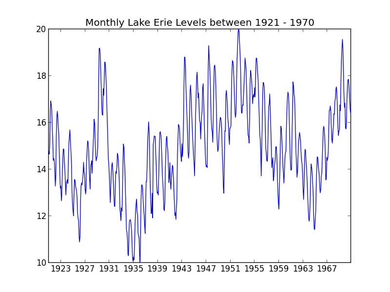
We first subtract off the linear term and ensure that the \(x\) axis is taking numerical values.
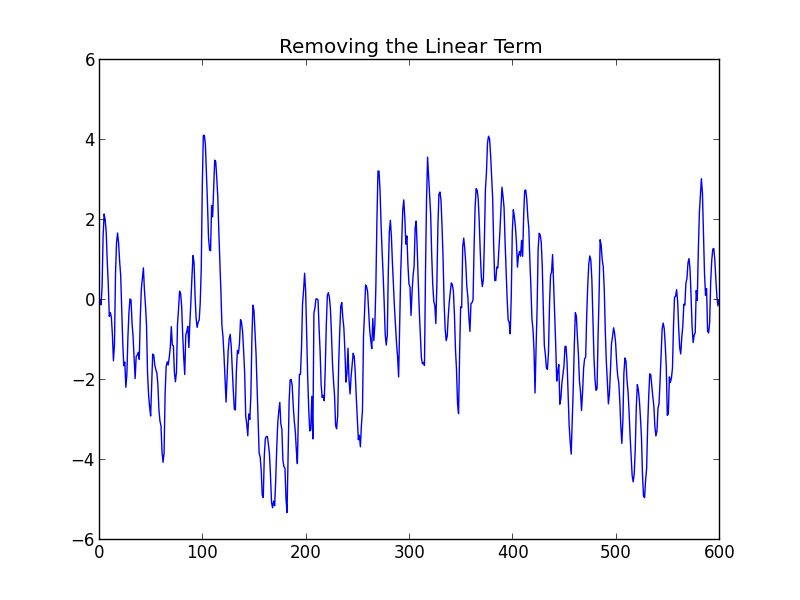
We perform the transformation using Eq 1 and plot the magnitude of the result.
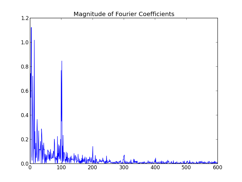
Notice that the first 100 or so terms drop off very quickly and then the terms more-or-less flatten out. This is where we will cut off the series.
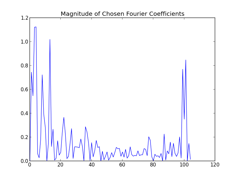
Here we have kept 120 coefficients. The need to keep even this many (vs the 600 that we originally computed) is because our data set is not great (by this, I mean it actually contains some high frequency components that are not merely noise.). However, the exact number of terms is not critical. A few extra terms will not have a profound effect on the result.
We truncate the series after the first 120 terms and arrive at the smoothed fit
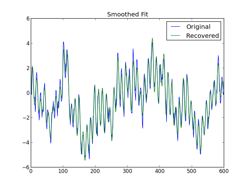
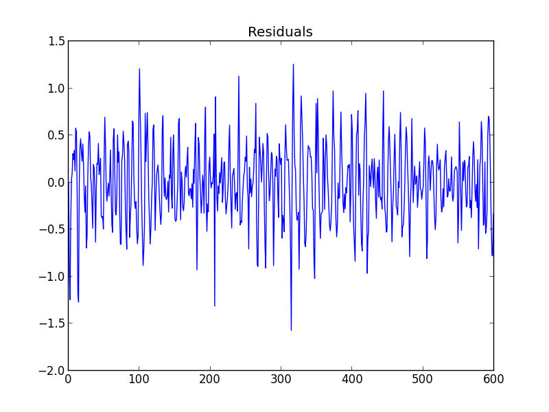
and residuals.
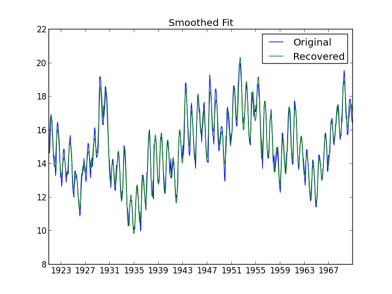
Adding back the linear term we get the smoothed fit to the original data.
Additional Note
I think it’s important to mention the fact that if, after smoothing our data, we then wish to find an approximation to the derivative of the underlying process, we should NOT simply take the derivative of the smoothed approximation (2). Several higher order terms were dropped in (2) and the derivative is not as smooth as our original function. Therefore it is reasonable to expect that we will need to keep more terms in the Fourier series of the derivative. To put it simply: the derivative of a good approximation is not necessarily a good approximation to the derivative.
The derivative by definition is concerned with the immediate vicinity of our data points. So a better solution to the problem is to use a method similar to the one outlined in my previous post and just use the \(k\) closest neighbors to each data point to compute an approximation to the derivative.