Differentiation by Integration Part III
This post is the final in a series of posts on an interesting method for finding the derivative of a function, either empirical or otherwise, using integration. You can see the empirical formula here and the analytical version here. Here we will be visualizing the results developed previously.
First Example
For the first example, consider the simple function
\[y = 5x^2\]which describes the position of a particle moving on a line with constant acceleration. We also admit that we have noisy measurements.
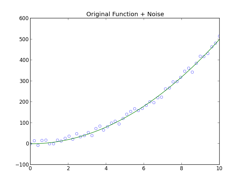
In practice we only have these measurements (the open circles), however here I have included the theoretical model.
The problem now is to get an estimate of the derivative from the measurements. The presence of noise compounds the problem as is illustrated by using a simple difference formula
\[f'(x) = \frac{f(x+h) - f(x)}{h}.\]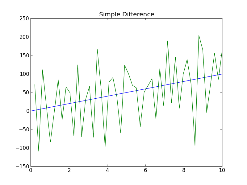
Here, I have included the theoretical value for the derivative since it is simple to compute in this example.
A much smoother and more accurate formula is given by formula (3) in this post.
\[f'(x) = \frac{\sum_{\alpha=-k}^k\alpha f(x+\alpha h)}{2 \sum_{\alpha = 1}^k \alpha^2h}\]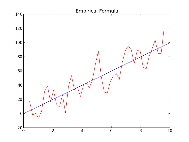
Side-by-side the difference is obvious.
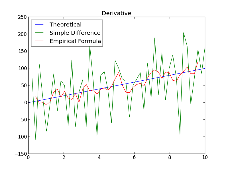
Finally, equation (2) from my original post on this topic provides an analytical approximation to the derivative.
\[\begin{align*} f'(x) &= \frac{3}{2 \varepsilon^3} \int_{-\varepsilon}^{\varepsilon}tf(x + t) ~ dt\\ &= \frac{3}{2 \varepsilon^3}5 \int_{-\varepsilon}^{\varepsilon}t(x+t)^2 ~dt\\ &= 10x. \end{align*}\]In fact, it gives the exact value for the derivative! This is expected since all the terms above second order in the Taylor series expansion of our function, \(f\) are zero.
A Second Example
Now consider samples taken from a process expected to follow the relationship
\[y = \cos x.\]Where again we have noise on our measurements.
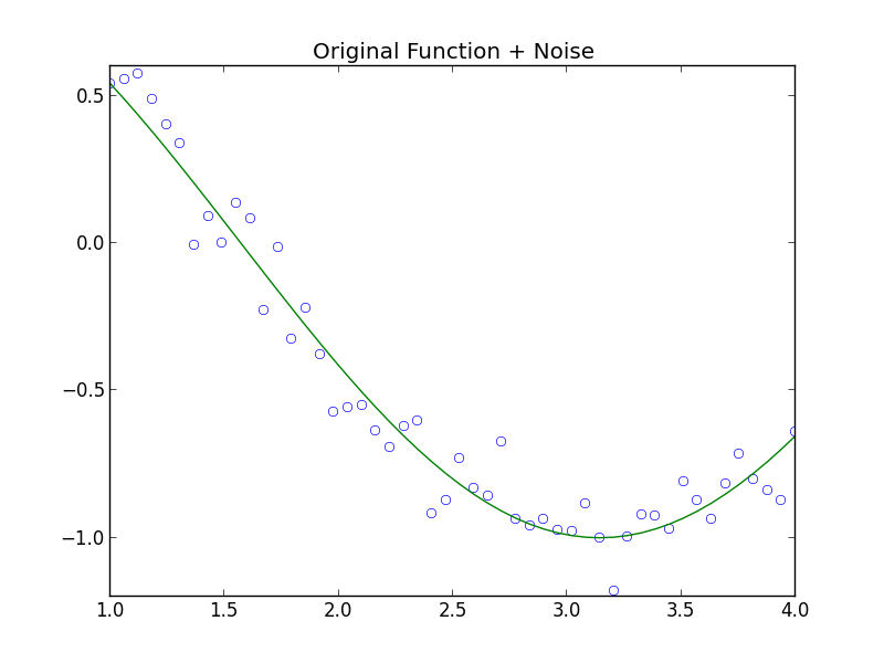
The next plot shows how the first two approximations above match the known derivative of our model.
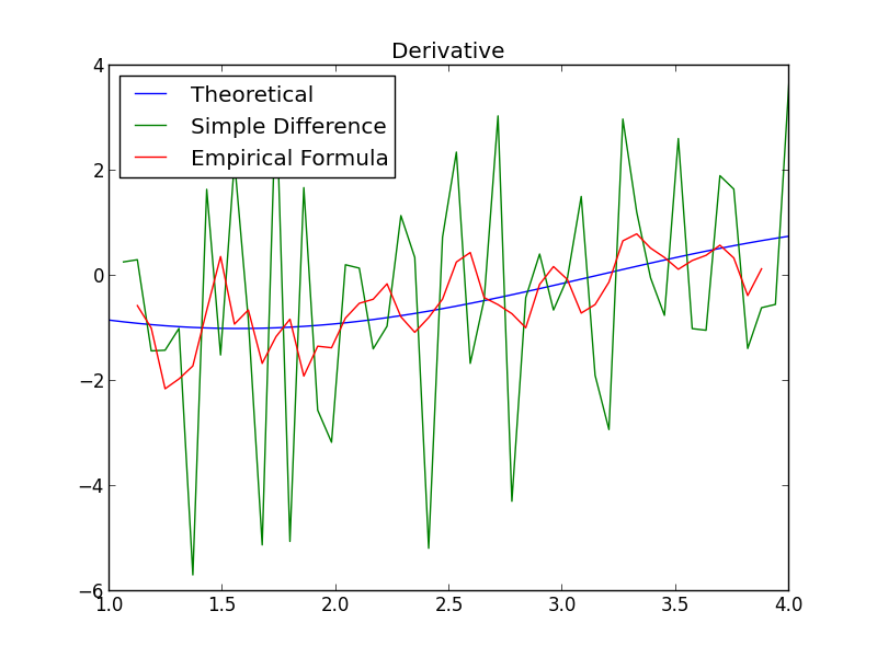
This time, the analytical formula does not provide the exact value of the derivative at our data points, but rather an approximation that depends on the parameter \(\varepsilon\):
\[\begin{align*} f'(x) &= \frac{3}{2 \varepsilon^3} \int_{-\varepsilon}^{\varepsilon}tf(x + t) ~ dt\\ &= \frac{3}{2 \varepsilon^3} \int_{-\varepsilon}^{\varepsilon}t\cos(x + t) ~ dt\\ &= \frac{3}{2 \varepsilon^3} \int_{-\varepsilon}^{\varepsilon}t\cos(t)\cos(x) - t\sin(t)\sin(x)~ dt\\ &= \frac{3}{\varepsilon^3}(\varepsilon\cos\varepsilon - \sin \varepsilon)\sin x. \end{align*}\]Below is a plot of the known derivative along with the above approximation with several values for the parameter \(\varepsilon\).
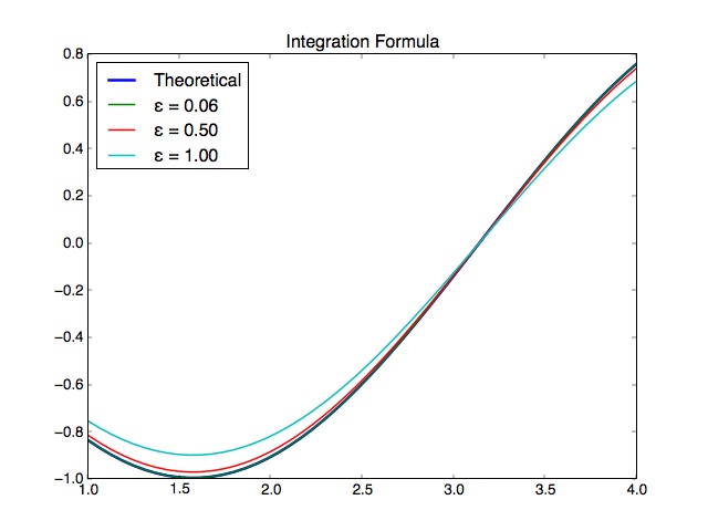
Note that the value \(\varepsilon = 0.06\) corresponds with the distance between the data points in the second example. At this value of \(\varepsilon\), the true derivative and the approximation are nearly indistinguishable.