Approximating Traffic Speed with Fourier Analysis
Here, we look at a simple model for traffic speed on the streets of San Francisco. We’re only going to look at a single street over the course of a week. At the end, we will discuss the short-comings (they are obvious) as well as consider important characteristics that should be captured by a better model.
The data was taken from Caltrans PeMS. For the purpose of this post, we are using the hourly aggregate data. Here is a sample from station id 400043.
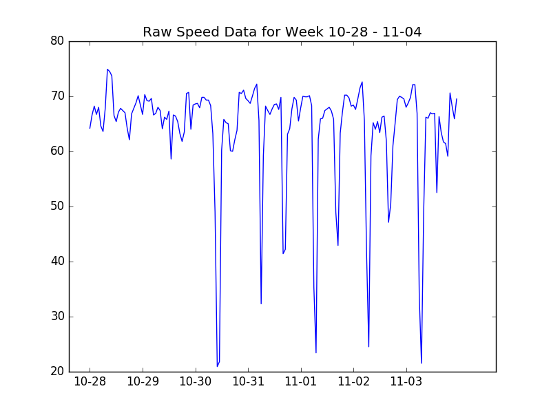
From this, it is obvious that there is a periodic component to the data. This leads us to suspect a Fourier representation would be a good place to start. Something of the form:
\[\begin{equation} \hat{y}(t) = c+ \sum_i \left[a_i\sin(2\pi\nu_i t) + b_i\cos(2\pi \nu_it)\right] \end{equation}\]We can guess at the frequencies, $\nu_i$ that would make the most sense. But this may lead to disagreement. Instead, we can look at the power spectrum in the frequency space over a larger sample of the data.
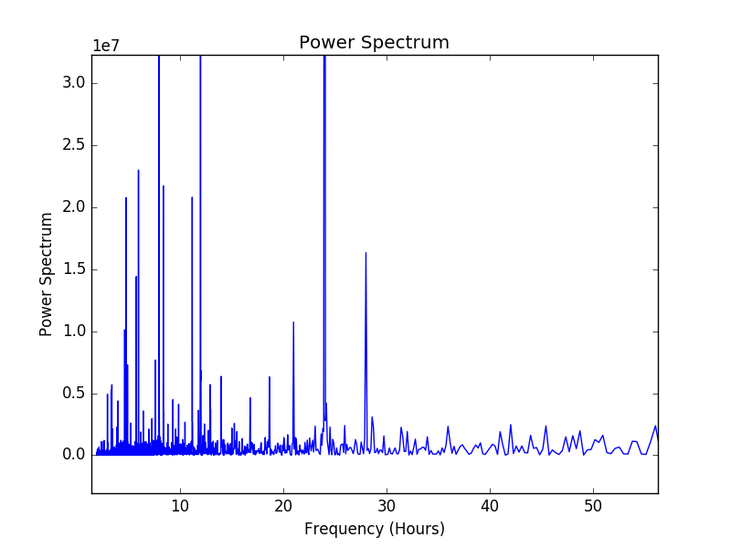
Here, I used numpy’s fft package and ignored all the negative frequencies. In the above plot, we notice a large spike at a 24 hour (daily) frequency. From my own experiments, using this one frequency actually provides the best fit in this case. Then our model (1) simply becomes
\[\hat{y}(t) = c+ a_i\sin\left(\frac{2\pi t}{24}\right) + b_i\cos\left( \frac{2\pi t}{24}\right)\]Then, we can use the principle of least squares to fit this model to a year’s worth of data. The result of this fit compared to a test week is shown in the next plot.
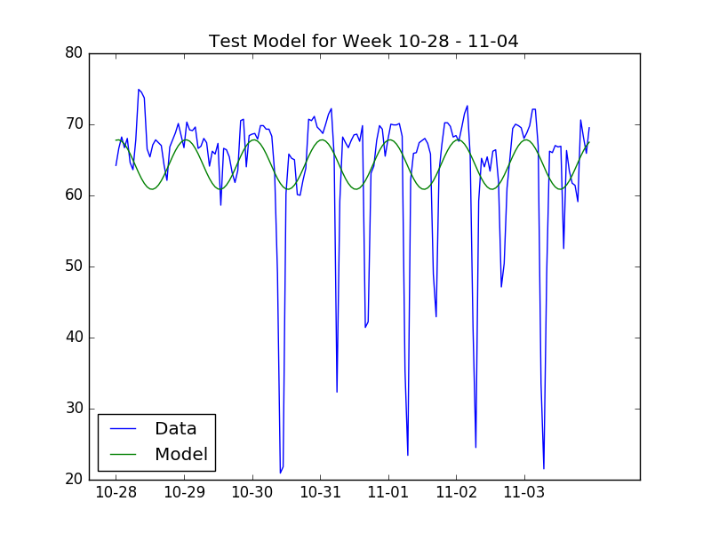
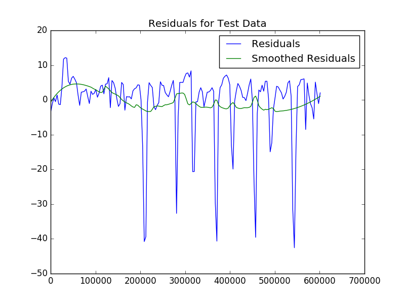
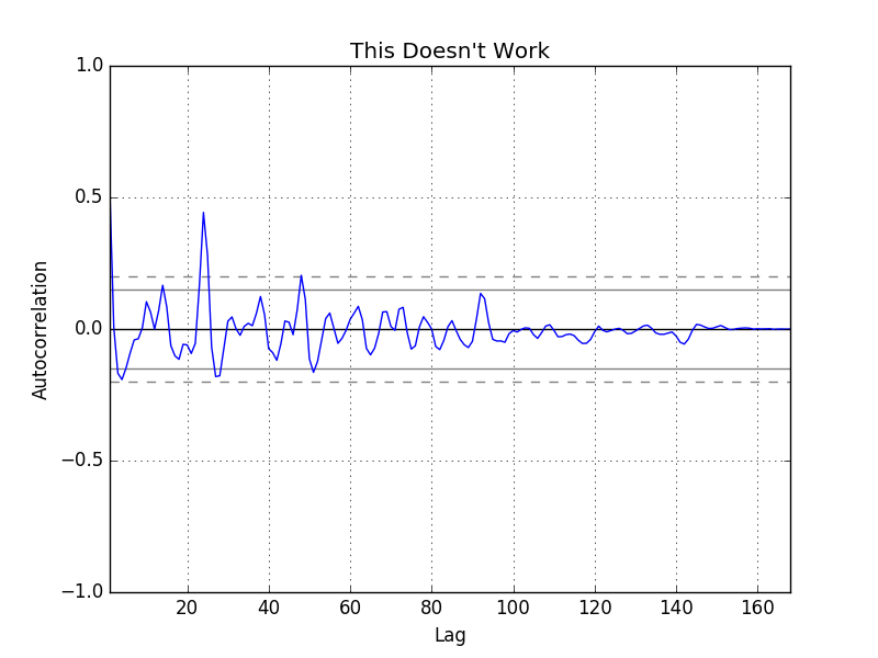
From this plot, we see that the daily changes in traffic speed are captured. However, there are glaring holes in the model as it misses the large downward spikes that happen nearly every day. I looked at the auto-correlation of the residuals, but this proved to not be as useful as I had hoped
Short-comings
As I said at the outset, this model has several short-comings. To name two:
-
It does not capture shocks in speed. Traffic flow is not a linear process. As evidenced by the plots above, there are regular shocks to the traffic flow. These occur at nearly periodic intervals. These near periodicity suggests a chaotic element to the process. However, I would need to look at this more (and perhaps at more granular data) because the power spectrum is not as dense as I would expect for a chaotic system.
-
The model does not take neighboring roads into account This is easy to overcome, but as is, there is no connection between neighboring roads incorporated in the model.
How is this helpful?
Though this model has obvious short-comings. I think it does provide evidence for the assumptions that have been used in other models I have read about. In particular, it is obvious from my model that the traffic process mostly just repeats itself every day.
Possible improvements
Kwon and Murphy have propsed a Coupled Hidden Markov Model for the traffic process. While this captures some of the dynamics present in the system, it has several shortcomings. Possibly the most serious is that traffic is not a Markov process. That is, to be able to predict what state the traffic will be in in the next time step, it is not sufficient to only know the current state. For this reason, the ability to make reasonable predictions about the state of traffic in the future is lacking in their model.
Another model I have seen is the MIT Radiation model (sorry, when I wrote this article, a direct link to the lab was broken. The lab was here.) There model has the obvious advantage of being graphically based and thus capturing the connections between road segments.
As mentioned earlier, traffic is clearly a non-linear process. Researchers at MIT have been working on traffic models using non-linear dynamics.