Detecting Step Edges in a Time Series
Edge detection is a preliminary step in many computer vision algorithms. In particular, a step edge is an important feature of an image to identify. Here, I will outline John Canny’s 1986 paper, “A Computational Approach to Edge Detection”. I will focus, as Canny does in most of his paper, on a one dimensional edge. This corresponds to detecting a mean shift or step edge in a time series.
There are three criteria that we will consider in judging whether our edge detector is a success:
- Good detection – There should be a low probability of failing to mark real edge points as well as a low probability of marking points that are not edges. This goal is reached by maximizing the output signal-to-noise ratio.
- Good localization – The points marked as edge points should be as close as possible to the true edge.
- Only one response per edge – This is implicit in the first criteria. If we get multiple responses for a single edge we are obviously marking non-edge points as belonging to an edge. However, this points needs to be made explicit due to the mathematical formulation to follow.
Detection and Localization Criteria
We now look at how to formalize the first two criteria above. We will begin with a step edge, \(G(x)\) in white Gaussian noise, \(n(x)\). For simplicity, we will assume the step is centered at \(x=0\). We will then form the convolution of \(G(x)\) and the filter we are yet to discover whose impulse response will be denoted by, \(f(x)\). A local maximum of this convolution will denote the center of the edge we hope to detect. Our work now is to find the ideal filter.
The response of the filter to the step edge will be denoted by \(H_G\) and is given by the convolution integral:
\[H_G = \int_{-W}^WG(-x)f(x)\,dx\]assuming the filter has a finite impulse response on the window, \([-W,W]\). The root-mean-squared response to the noise is
\[H_n = n_0\int_{-W}^Wf(x)\,dx\]where \(n_0^2\) is the mean-squared amplitude of the noise. With these definitions, it is clear that we can achieve condition (1) above if we optimize the signal-to-noise ratio defined by
\[\mathsf{SNR} = \frac{\left| \int_{-W}^W G(-x)f(x) \,dx \right|}{n_0\sqrt{\int_{-W}^W f^2(x)\,dx}}\]To achieve the second criterion we will use the reciprocal of the root-mean-square distance of the marked edge from the true edge. Since we are looking at local maxima of the convolution, the first derivative of the response will be zero at these points. Recall that we are assuming a step edge at \(x=0\). Then in the absence of noise, we expect a local maximum in the response at \(x=0\).
Let \(H_n(x)\) be the response of the filter to random noise and \(H_G(x)\) the response to the edge. Suppose there is a local maximum in the total response at \(x=x_0\). Then
\[H'_G(x_0) + H'_n(x_0) = 0.\]The Taylor expansion of \(H'_G(x_0)\) about the origin is
\[H'_G(x_0) = H'_G(0) + H''_G(0)x_0 + O(x_0^2).\]By assumption \(H'_G(0) = 0\) and if \(x_0\) is small, we can ignore the last quadratic term. This gives us the equation
\begin{equation} H’'_G(0)x_0 \approx -H’_n(x_0). \end{equation}
\(H'_n(x_0)^2\) is a Gaussian random quantity whose variance is given by
\[E[H'_n(x_0)^2] = n_0^2 \int_{-W}^W f'^2(x)\,dx.\]Where \(E[y]\) is the expected value of \(y\). Then from Eq (1) above we get
\[x_0^2 \approx \frac{-H'^2_n(x_0)}{H''^2_G(0)}\]and substituting for \(H_G\) we get for all \(x_0 \approx 0\)
\[E[x_0^2] \approx \frac{n_0^2 \int_{-W}^W f'^2(x)\,dx}{\left[\int_{-W}^W G'(-x)f'(x)\,dx\right]^2}.\]The square-root of the inverse of this last expression is what we will use as our definition of localization:
\[\mathsf{Localization} = \frac{\left| \int_{-W}^W G'(-x)f'(x) \,dx \right|}{n_0\sqrt{\int_{-W}^W f'^2(x)\,dx}}.\]Simultaneously optimizing the SNR and Localization as defined above allows us to meet the first two criteria set out in the first section. Although any monotonic combination of these functions would be sufficient, we will choose to optimize their product
\[\frac{\left| \int_{-W}^W G(-x)f(x) \,dx \right|}{n_0\sqrt{\int_{-W}^W f^2(x)\,dx}}\frac{\left| \int_{-W}^W G'(-x)f'(x) \,dx \right|}{n_0\sqrt{\int_{-W}^W f'^2(x)\,dx}}.\]There may be additional restraints that need to be imposed on the problem such as the multiple edge criteria which we will discuss next.
Eliminating Multiple Responses
We need an expression for the distance between peaks. It should be clear that the mean distance between peaks in the output will be twice the distance between zero-crossings in the derivative. Then we can make use of a result formulated by Rice that the average distance between zero-crossings of the response of a function \(g\) to Gaussian noise is
\[x_{ave} = \pi \left( \frac{-R(0)}{R''(0)}\right)^{1/2}\]where \(R(g)\) is the autocorrelation of \(g\). Here, we are looking for the mean zero-crossing spacing for \(f'\). Making use of Rice’s result we have
\[x_{zc}(f') = \pi \left(\frac{\int_{-\infty}^{+\infty}f'^2(x)\,dx}{\int_{-\infty}^{+\infty}f''^2(x)\,dx}\right)^{1/2}\]As noted above, the difference between adjacent maxima, \(x_{max}\) will be twice \(x_{zc}\). We set this equal to some multiple \(k\) of the width of our operator, \(W\)
\[x_{max} = 2x_{zc} = kW.\]This final equation can then be used quite naturally to control the number of maxima due to noise, \(N_n\)
\[N_n = \frac{2W}{x_{max}} = \frac{2}{k}.\]Fixing \(k\) fixes the number of maxima in the response attributed to noise.
Approximating Optimal Detectors
In general, it will be difficult or impossible to find an optimal solution to our problem satisfying a constraint such as the multiple response constraint. Instead, you can use what Canny refers to as a penalty method, or in the language of modern machine learning, regularization. Instead of optimizing your desired functional with constraints, \(P_i\), we can instead optimize their linear combination:
\[J(f) = \mathsf{SNR}(f)\times \mathsf{Localization}(f) + \sum\mu_i P_i\]I will leave out the details that Canny works through to find a numerical solution to the problem of detecting edge signals. I included a brief discussion about the penalty method simply due to the ubiquity and useful of this technique. Instead I want to concentrate on a useful approximation to the optimal detector.
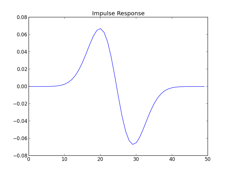
The approximation that Canny notes is the first derivative of a Gaussian
\begin{equation} f(x) = -\frac{x}{\chi^2}\exp\left(-\frac{x^2}{\sigma^2}\right) \end{equation}
He admits that the results are about 20% worse with this filter than that of the optimal filter. However, the advantages of using a derivative of a Gaussian come in the ease of computation, especially in higher dimensions. Of particular interest is the 2D case for detecting edges in images.
Below we use this \(f\) in an example.
An Example
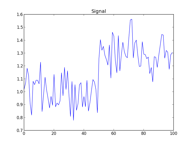
For a quick example, we have a signal with a single step.

We take as our filter, the one whose impulse response is the first derivative of a Gaussian.

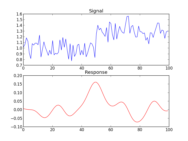
Taking the maximum of the convolution between our signal and the filter provides the location of the center of the step.

A Note about Width
As I tinkered with the above approach for step detection, I realized that as with several algorithms, the width of the filter changes the results significantly. Canny recommends using several different widths to find the response that best describes the signal you are working within each localized area of the signal. Indeed, the ideal width of the operator is dependent on the (local) SNR of the signal. Specifically, if we can model the noise energy by a known probability distribution we can effectively calculate the probability that our detected edge is a true or spurious one. Note that this probability changes with the operator width given a fixed edge.