Solving a System of Coupled Differential Equations Using Matrix Algebra
A system of differential equations is said to be coupled if knowledge of one variable depends upon knowing the value of another variable. Examples include
- \[\begin{cases} \frac{dx}{dt} & = 3x^3 + 2y\\ \frac{dy}{dt} &= xyz\\ \frac{dz}{dt} &= x + 2y + z^2 \end{cases}\]
- \[\begin{cases} \frac{dx}{dt} & = e^y + 4\\ \frac{dy}{dt} &= \log x - y \end{cases}\]
- \[\begin{cases} \frac{dx}{dt} & = x + y\\ \frac{dy}{dt} &= 2x + 3y \end{cases}\]
Here we will discuss one method of solving a system of linear differential equations such as those in example (3) above.
To this end, we will employ the matrix notation
\[\begin{equation} \mathbf{x}' = A\mathbf{x} \end{equation}\]where
\[\mathbf{x} = \left(\begin{matrix} x_1\\ x_2\\ \vdots\\ x_n \end{matrix}\right)\]One solution is to immediately write down
\[\mathbf{x} = e^{At}\mathbf{x}_0\]but this requires knowledge of how to compute a matrix exponential
\[e^B = \sum_{k=0}^{\infty}\frac{1}{k!}B^k\]Another approach makes use of several tools learned in an introductory linear algebra class. To start we diagonalize the matrix \(A\) in equation (1).
\[A = P^{-1}DP\]Here, \(P\) is a matrix whose columns are the eigenvectors of \(A\) and \(D\) is a diagonal matrix whose entries are the corresponding eigenvalues of \(A\).
Then we can re-write Eq (1) as
\[\mathbf{x}' = P^{-1}DP\mathbf{x}\]and then observe that the system
\[\left(P\mathbf{x}\right)' = D\left(P\mathbf{x}\right)\]is a system of uncoupled differential equations of the variables \(P\mathbf{x}=\mathbf{y}\). These can be solved and
\[\mathbf{x}=P^{-1}\mathbf{y}.\]##Example
We will use the above method to solve the system of equations
\[\begin{cases} \frac{dx}{dt} &= y\\ \frac{dy}{dt} &= x \end{cases}\]This is re-written in matrix form (1) above where
\[A = \left( \begin{matrix} 0 & 1\\ 1 & 0 \end{matrix}\right)\]and
\[\mathbf{x} = \left(\begin{matrix} x\\ y \end{matrix}\right)\]To diagonalize \(A\) we need to calculate the eigenvectors of \(A\). To this end, we find the eigenvalues by solving the characteristic function
\[\begin{align*} \det\left(A-\lambda I\right) &= 0\\ \implies \lambda^2 - 1 &= 0 \end{align*}\]so that \(\lambda = \pm 1\). Then we can find the corresponding eigenvectors using the equation \(A\mathbf{x} = \lambda \mathbf{x}\) for each of the eigenvalues, \(\lambda\).
For \(\lambda = 1\),
\[\begin{equation} \left( \begin{matrix} 0 & 1\\ 1 & 0 \end{matrix}\right)\left(\begin{matrix} x\\ y \end{matrix}\right)= \left(\begin{matrix} x\\ y \end{matrix}\right) \end{equation}\] \[\implies x = y\]So that the eigenvector associated with the first eigenvalue is
\[\mathbf{x} = \left(\begin{matrix} 1\\ 1 \end{matrix}\right).\]Similarly, the eigenvector corresponding with the eigenvalue \(\lambda = -1\) is
\[\mathbf{x} = \left(\begin{matrix} 1\\ -1 \end{matrix}\right).\]These lead us to the following definitions for matrices \(P\) and \(D\) above,
\[P = \left(\begin{matrix} 1 & 1\\ 1 & -1 \end{matrix}\right)\] \[D = \left(\begin{matrix} 1 & 0\\ 0 & -1 \end{matrix}\right)\]So our system of decoupled differential equations is
\[\begin{align*} \left(P\mathbf{x}\right)' &= D\left(P\mathbf{x}\right)\\ \left(\begin{matrix} u\\ v \end{matrix}\right)' &= \left(\begin{matrix} 1 & 0\\ 0 & -1 \end{matrix}\right)\left(\begin{matrix} u\\ v \end{matrix}\right) \end{align*}\]where
\[\begin{align*} \left(\begin{matrix} u\\ v \end{matrix}\right) &= P\mathbf{x}\\ &= \left(\begin{matrix} 1 & 1\\ 1 & -1 \end{matrix}\right)\left(\begin{matrix} x\\ y \end{matrix}\right)\\ &= \left(\begin{matrix} x + y\\ x - y \end{matrix}\right) \end{align*}\]Writing out our new system of equations we see
\[\begin{align*} u' &= u\\ v' &= v \end{align*}\]which quickly leads to the solutions
\[\begin{align} u &= C_1e^t\\ v &= C_2e^{-t} \end{align}\]To get our solution in terms of \(\mathbf{x}\) we need to apply \(P^{-1}\) to our solution
\[P^{-1} = \frac{1}{2}\left(\begin{matrix} -1 & -1\\ -1 & 1 \end{matrix}\right)\]Doing this we get
\[\begin{align*} \mathbf{x} &= P^{-1}\mathbf{y}\\ &= \frac{1}{2}\left(\begin{matrix} -1 & -1\\ -1 & 1 \end{matrix}\right) \left(\begin{matrix} u\\ v \end{matrix}\right)\\ &= \frac{1}{2} \left(\begin{matrix} -C_1e^t - C_2e^{-t}\\ -C_1e^t + C_2 e^{-t} \end{matrix}\right) \end{align*}\]By redefining our constants \(C_1 \equiv \frac{1}{2}C_1\) and \(C_2 \equiv \frac{1}{2}C_2\) we get our solutions to the original set of coupled differential equations to be
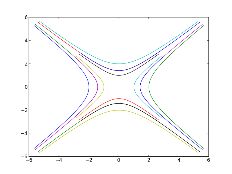
\[\begin{align} x &= C_1e^t + C_2e^{-t}\\ y &= C_1e^t - C_2e^{-t} \end{align}\]Below is a plot of these solutions for different combinations of \(C_1\) and \(C_2\) both varying between -1 and 1 and \(-1.7 \le t\le 1.7\).

This is a technique used in a lot of physics and engineering problems that a student in a beginning linear algebra class could understand (given a basic calculus background that most would be expected to have in such a course). I also feel it could be another good way to answer a question of the form “what is this good for?” Perhaps if I teach again.