Saddle-node Bifurcations
Often, a non-linear dynamical system will depend on a parameter. The value of which can drastically affect the long term behavior of the system. As a simple example consider the system
\[\begin{equation} \dot{x} = r + x^2 \end{equation}\]Notice that as the value of the parameter $r$ is varied, the fixed points of the system change
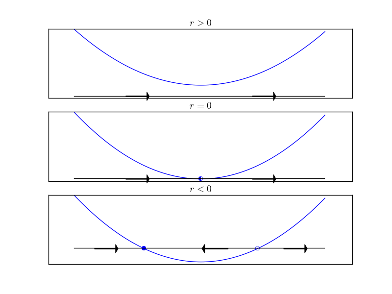
How parameters affect a system is the topic of study in bifurcation theory. Notice in the figure above that when $r \gt 0$ there are no fixed-points. As $r$ decreases, first a “half-stable” fixed point appears at $x=0$, and then two distinct fixed points emerge seemingly out of nowhere (this description has lead some to call this type of bifurcation a “blue sky” bifurcation). We will call this type of bifurcation a saddle-node bifurcation.
There are several ways to visualize how the fix points of a system depend on the parameter $r$. The figure above is one example. It is also more convenient to omit the plot of $\dot{x}$ above the $x$-axis.
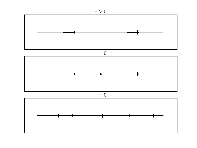
(Personally, this is my favorite visualization as it is easy to generate these plots.)
If we look at the fixed points of the system (1), $x^*$ they will solve the equation
\[0 = r + x^2\]So that
\[r = -{x^*}^2\]Which is a simple plot. However, it is preferable to look at the this image with the axes inverted. This makes it clear that the fixed points of the system, $x^*$ are a function of the parameter, $r$.
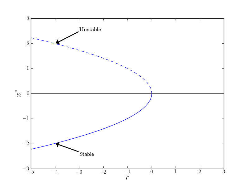
Here, it is often useful to make use of your favorite plotting software rather than drawing these graphs by hand. Wolfram Alpha works very well if nothing else is available.
Another Example
Consider the system
\[\begin{equation} \dot{x} = r + x - \log(1+x) \end{equation}\]Since the shape of the system isn’t immediately clear we can instead plot the simpler functions $r + x$ and $\log(1+x)$. Where the two graphs intersect are the fixed points of the system since $r + x^* = \log(1+x^*)$ at these points. When $r+x$ is above $\log(1+x)$ the flow is to the right and when the line is below $\log(1+x)$ the flow is to the left.
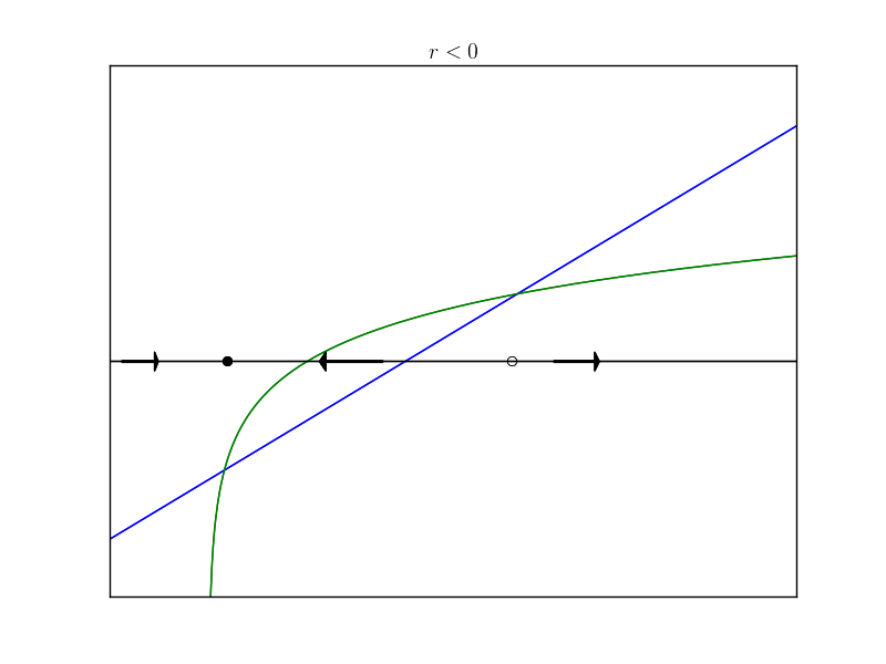
Again, at some $r_c$ the two two curves will intersect tangentially indicating a “half-stable” fixed point.
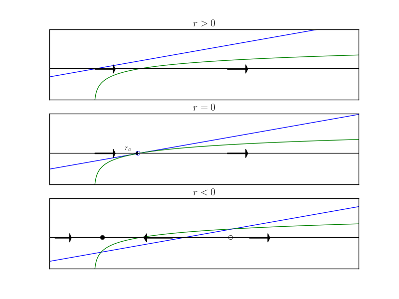
We can calculate the value of $r_c$ by requiring the equality of the functions as well as the derivative (since they intersect tangentially).
\[\begin{align} r + x &= \log(1+x) \\ 1 &= \frac{1}{1+x} \end{align}\]From (4) we get, $x=0$. Substituting this into (3) we get
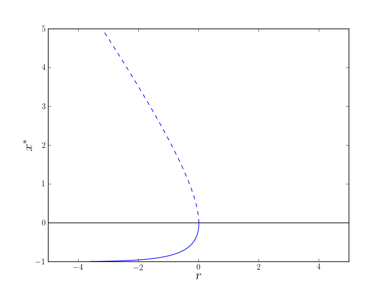
\[r_c = 0.\]To make the bifurcation diagram, notice that it is much easier (i.e. possible) to solve for $r$ as a function of $x$ than the other way around. For a fixed point, $x^*$
\[r = \log(1+x^*) - x^*\]Then we can just switch $x$ and $r$ in our plotting software (I’m using Matplotlib) to get our bifurcation diagram.
Normal Forms
Above, we said that (1) was a “simple” example. Actually, (1) is the prototypical example of a saddle-node bifurcation. Indeed, (1) is the normal form for this type of bifurcation. By normal form we mean that all saddle-node bifurcations look like (1) at least locally (i.e. if you “zoom in” enough).